Optimization
Contents:
Introduction
Recall that the linear function had the form \(f(x_i, W) = W x_i\) and the SVM we developed was formulated as:
Optimization is the process of finding the set of parameters \(W\) that minimize the loss function.
Non-differentiable loss functions. As a technical note, you can also see that the kinks in the loss function (due to the max operation) technically make the loss function non-differentiable because at these kinks the gradient is not defined. However, the subgradient still exists and is commonly used instead. In this class will use the terms subgradient and gradient interchangeably.
Optimization
To reiterate, the loss function lets us quantify the quality of any particular set of weights \(W\). The goal of optimization is to find \(W\) that minimizes the loss function.
Strategy #3: Following the Gradient
It turns out that there is no need to randomly search for a good direction: we can compute the best direction along which we should change our weight vector that is mathematically guaranteed to be the direction of the steepest descend (at least in the limit as the step size goes towards zero). This direction will be related to the gradient of the loss function.
In one-dimensional functions, the slope is the instantaneous rate of change of the function at any point you might be interested in. The gradient is a generalization of slope for functions that don’t take a single number but a vector of numbers. Additionally, the gradient is just a vector of slopes (more commonly referred to as derivatives) for each dimension in the input space. The mathematical expression for the derivative of a 1-D function with respect its input is:
When the functions of interest take a vector of numbers instead of a single number, we call the derivatives partial derivatives, and the gradient is simply the vector of partial derivatives in each dimension.
Computing the gradient
There are two ways to compute the gradient: A slow, approximate but easy way (numerical gradient), and a fast, exact but more error-prone way that requires calculus (analytic gradient).
Computing the gradient numerically with finite differences
This means iterates over all dimensions one by one, makes a small change h along that dimension and calculates the partial derivative of the loss function along that dimension by seeing how much the function changed. The variable grad holds the full gradient in the end.
Note that in the mathematical formulation the gradient is defined in the limit as \(h\) goes towards zero, but in practice it is often sufficient to use a very small value (such as 1e-5). Ideally, you want to use the smallest step size that does not lead to numerical issues. Additionally, in practice it often works better to compute the numeric gradient using the centered difference formula (wiki): \([f(x+h) - f(x-h)] / 2 h\).
Update in negative gradient direction. After computing a gradient update should be done in negative direction.
Effect of step size. The gradient tells us the direction in which the function has the steepest rate of increase, but it does not tell us how far along this direction we should step. As we will see later in the course, choosing the step size (also called the learning rate) will become one of the most important hyperparameter settings in training a neural network.
A problem of efficiency. You may have noticed that evaluating the numerical gradient has complexity linear in the number of parameters. In our example we had 30730 parameters in total and therefore had to perform 30,731 evaluations of the loss function to evaluate the gradient and to perform only a single parameter update. This problem only gets worse, since modern Neural Networks can easily have tens of millions of parameters.
Computing the gradient analytically with Calculus
The numerical gradient is very simple to compute using the finite difference approximation, but the downside is that it is approximate (since we have to pick a small value of h, while the true gradient is defined as the limit as h goes to zero), and that it is very computationally expensive to compute. The second way to compute the gradient is analytically using Calculus, which allows us to derive a direct formula for the gradient (no approximations) that is also very fast to compute. However, unlike the numerical gradient it can be more error prone to implement, which is why in practice it is very common to compute the analytic gradient and compare it to the numerical gradient to check the correctness of your implementation. This is called a gradient check.
Lets use the example of the SVM loss function for a single datapoint:
We can differentiate the function with respect to the weights. For example, taking the gradient with respect to \(w_{y_i}\) we obtain:
where \(\mathbb{1}\) is the indicator function that is one if the condition inside is true or zero otherwise. While the expression may look scary when it is written out, when you’re implementing this in code you’d simply count the number of classes that didn’t meet the desired margin (and hence contributed to the loss function) and then the data vector \(x_i\) scaled by this number is the gradient. Notice that this is the gradient only with respect to the row of \(W\) that corresponds to the correct class. For the other rows where \(j \neq y_i\) the gradient is:
Once you derive the expression for the gradient it is straight-forward to implement the expressions and use them to perform the gradient update.
Gradient Descent
Now that we can compute the gradient of the loss function, the procedure of repeatedly evaluating the gradient and then performing a parameter update is called Gradient Descent. Its vanilla version looks as follows:
while True:
    weights_grad = evaluate_gradient(loss_fun, data, weights)
    weights += - step_size * weights_grad # perform parameter update
Mini-batch gradient descent. The training data can have on order of millions of examples. Hence, it seems wasteful to compute the full loss function over the entire training set in order to perform only a single parameter update. A very common approach to addressing this challenge is to compute the gradient over batches of the training data. The reason this works well is that the examples in the training data are correlated.
The extreme case of this is a setting where the mini-batch contains only a single example. This process is called Stochastic Gradient Descent (SGD) (or also sometimes on-line gradient descent).
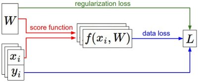
Summary of the informational flow. During the forward pass the score function computes class scores, stored in vector f. The loss function contains two components: The data loss computes the compatibility between the scores f and the labels y. The regularization loss is only a function of the weights. During Gradient Descent, we compute the gradient on the weights (and optionally on data if we wish) and use them to perform a parameter update during Gradient Descent.