Backpropagation
Contents
Introduction
In this section we will develop expertise with an intuitive understanding of backpropagation, which is a way of computing gradients of expressions through recursive application of chain rule.
The core problem studied in this section is as follows: We are given some function \(f(x)\) where \(x\) is a vector of inputs and we are interested in computing the gradient of \(f\) at \(x\) (i.e. \(\nabla f(x)\) ).
Simple expressions and interpretation of the gradient
where derivatives indicate the rate of change of a function with respect to that variable surrounding an infinitesimally small region near a particular point:
A nice way to think about the expression above is that when \(h\) is very small, then the function is well-approximated by a straight line, and the derivative is its slope. In other words, the derivative on each variable tells you the sensitivity of the whole expression on its value.
As mentioned, the gradient \(\nabla f\) is the vector of partial derivatives, so we have that \(\nabla f = [\frac{\partial f}{\partial x}, \frac{\partial f}{\partial y}] = [y, x]\) Another operations may be also be derived:
Max function sensitive only to changing bigger value.
Compound expressions with chain rule
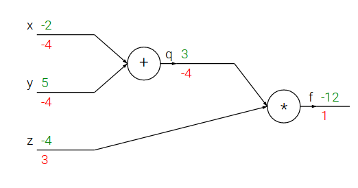
Lets now start to consider more complicated expressions that involve multiple composed functions, such as \(f(x,y,z)=(x+y)z\). Note that this expression can be broken down into two expressions: \(q=x+y\) and \(f=qz\). Moreover, we know how to compute the derivatives of both expressions separately, as seen in the previous section. \(f\) is just multiplication of \(q\) and \(z\), so \(\frac{\partial f}{\partial q} = z, \frac{\partial f}{\partial z} = q\), and \(q\) is addition of \(x\) and \(y\) so \(\frac{\partial q}{\partial x} = 1, \frac{\partial q}{\partial y} = 1\). The chain rule tells us that the correct way to “chain” these gradient expressions together is through multiplication. For example, \(\frac{\partial f}{\partial x} = \frac{\partial q}{\partial x} \frac{\partial f}{\partial q}\). In practice this is simply a multiplication of the two numbers that hold the two gradients.
# set some inputs
x = -2; y = 5; z = -4

# perform the forward pass
q = x + y # q becomes 3
f = q * z # f becomes -12

# perform the backward pass (backpropagation) in reverse order:
# first backprop through f = q * z
dfdz = q = 3
dfdq = z = -4

# now backprop through q = x + y
dfdx = dqdx * dfdq = 1 * -4 = -4
dfdy = dqdy * dfdq = 1 * -4 = -4
At the end we are left with the gradient in the variables [dfdx,dfdy,dfdz], which tell us the sensitivity of the variables x,y,z on f!.
Modularity: Sigmoid example
Let’s take a look to sigmoid activation function:
The function is made up of multiple gates. Here are the derivatives for them:
Where the functions \(f_c, f_a\) translate the input by a constant of \(c\) and scale the input by a constant of \(a\), respectively.
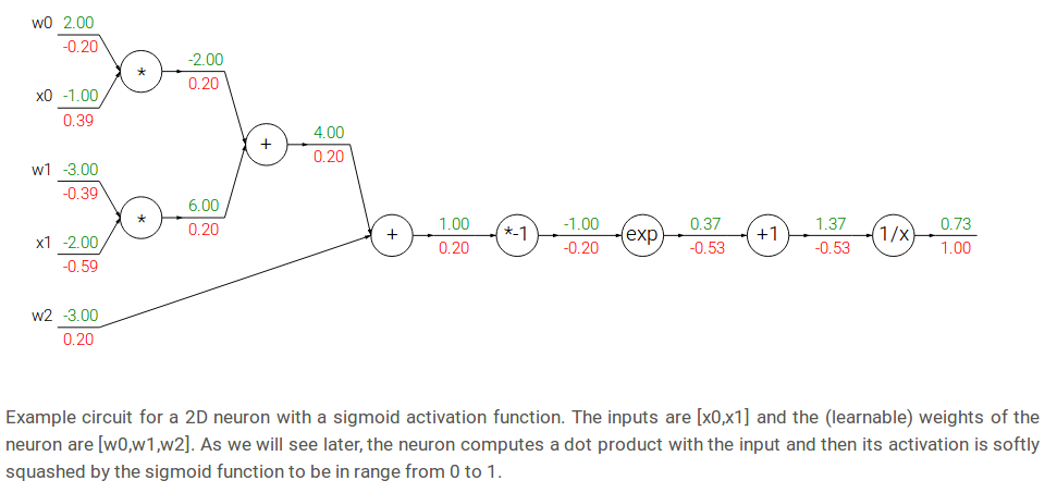
so, to apply chain rule we:
- Compute local derivative of the part of function according to it’s inputs
- Multiply local derivative to derivative from \(L_{i+1}\) layer
For example from circuit:
- for \(f(x) = e^x\) input was \(x=-1.0\), derivative at next layer \(\frac{dL_{i+1}}{dx} = -0.53\)
- derivative for \(L_i\) layer is \(\frac{df}{dx} = e^x = e^{-1} = 0.37\) (local derivative, not exist at picture)
- now to get gradient we should multiply local derivative with derivative from the next layer \(res = \frac{df}{dx} * \frac{dL_{i+1}}{dx} = 0.37 * -0.53 = -0.2\)
It turns out that the derivative of the sigmoid function with respect to its input simplifies if you perform the derivation:
As we see, the gradient turns out to simplify and becomes surprisingly simple. For example, the sigmoid expression receives the input 1.0 and computes the output 0.73 during the forward pass. The derivation above shows that the local gradient would simply be (1 - 0.73) * 0.73 ~= 0.2
w = [2,-3,-3] # assume some random weights and data
x = [-1, -2]

# forward pass
dot = w[0]*x[0] + w[1]*x[1] + w[2]
f = 1.0 / (1 + math.exp(-dot)) # sigmoid function

# backward pass through the neuron (backpropagation)
ddot = (1 - f) * f # gradient on dot variable, using the sigmoid gradient derivation
dx = [w[0] * ddot, w[1] * ddot] # backprop into x
dw = [x[0] * ddot, x[1] * ddot, 1.0 * ddot] # backprop into w
# we're done! we have the gradients on the inputs to the circuit
Implementation protip: staged backpropagation. As shown in the code above, in practice it is always helpful to break down the forward pass into stages that are easily backpropped through. For example here we created an intermediate variable dot which holds the output of the dot product between w and x. During backward pass we then successively compute (in reverse order) the corresponding variables (e.g. ddot, and ultimately dw, dx) that hold the gradients of those variables.
Backprop in practice: Staged computation
Suppose that we have a function of the form:
Forward pass:
x = 3 # example values
y = -4

# forward pass
sigy = 1.0 / (1 + math.exp(-y)) # sigmoid in numerator   #(1)
num = x + sigy # numerator                               #(2)
sigx = 1.0 / (1 + math.exp(-x)) # sigmoid in denominator #(3)
xpy = x + y                                              #(4)
xpysqr = xpy**2                                          #(5)
den = sigx + xpysqr # denominator                        #(6)
invden = 1.0 / den                                       #(7)
f = num * invden # done!                                 #(8)
Backward pass
# backprop f = num * invden
dnum = invden # gradient on numerator                             #(8)
dinvden = num                                                     #(8)
# backprop invden = 1.0 / den
dden = (-1.0 / (den**2)) * dinvden                                #(7)
# backprop den = sigx + xpysqr
dsigx = (1) * dden                                                #(6)
dxpysqr = (1) * dden                                              #(6)
# backprop xpysqr = xpy**2
dxpy = (2 * xpy) * dxpysqr                                        #(5)
# backprop xpy = x + y
dx = (1) * dxpy                                                   #(4)
dy = (1) * dxpy                                                   #(4)
# backprop sigx = 1.0 / (1 + math.exp(-x))
dx += ((1 - sigx) * sigx) * dsigx # Notice += !! See notes below  #(3)
# backprop num = x + sigy
dx += (1) * dnum                                                  #(2)
dsigy = (1) * dnum                                                #(2)
# backprop sigy = 1.0 / (1 + math.exp(-y))
dy += ((1 - sigy) * sigy) * dsigy                                 #(1)
# done! phew
Cache forward pass variables. To compute the backward pass it is very helpful to have some of the variables that were used in the forward pass. In practice you want to structure your code so that you cache these variables, and so that they are available during backpropagation.
Gradients add up at forks. The forward expression involves the variables \(x,y\) multiple times, so when we perform backpropagation we must be careful to use += instead of = to accumulate the gradient on these variables (otherwise we would overwrite it). This follows the multivariable chain rule in Calculus, which states that if a variable branches out to different parts of the circuit, then the gradients that flow back to it will add.
Patterns in backward flow
It is interesting to note that in many cases the backward-flowing gradient can be interpreted on an intuitive level. For example, the three most commonly used gates in neural networks (add,mul,max), all have very simple interpretations in terms of how they act during backpropagation.
The add gate always takes the gradient on its output and distributes it equally to all of its inputs, regardless of what their values were during the forward pass.
The max gate routes the gradient. Unlike the add gate which distributed the gradient unchanged to all its inputs, the max gate distributes the gradient (unchanged) to exactly one of its inputs (the input that had the highest value during the forward pass).
The multiply gate is a little less easy to interpret. Its local gradients are the input values (except switched), and this is multiplied by the gradient on its output during the chain rule.
Unintuitive effects and their consequences. Notice that if one of the inputs to the multiply gate is very small and the other is very big, then the multiply gate will do something slightly unintuitive: it will assign a relatively huge gradient to the small input and a tiny gradient to the large input. Note that in linear classifiers where the weights are dot producted \(w^T x_i\) (multiplied) with the inputs, this implies that the scale of the data has an effect on the magnitude of the gradient for the weights. For example, if you multiplied all input data examples \(x_i\) by 1000 during preprocessing, then the gradient on the weights will be 1000 times larger, and you’d have to lower the learning rate by that factor to compensate. This is why preprocessing matters a lot, sometimes in subtle ways! And having intuitive understanding for how the gradients flow can help you debug some of these cases.
Gradients for vectorized operations
Possibly the most tricky operation is the matrix-matrix multiplication (which generalizes all matrix-vector and vector-vector) multiply operations:
# forward pass
W = np.random.randn(5, 10)
X = np.random.randn(10, 3)
D = W.dot(X)

# now suppose we had the gradient on D from above in the circuit
dD = np.random.randn(*D.shape) # same shape as D
dW = dD.dot(X.T) #.T gives the transpose of the matrix
dX = W.T.dot(dD)
Tip: use dimension analysis! Note that you do not need to remember the expressions for dW and dX because they are easy to re-derive based on dimensions. For instance, we know that the gradient on the weights dW must be of the same size as W after it is computed, and that it must depend on matrix multiplication of X and dD (as is the case when both X,W are single numbers and not matrices). There is always exactly one way of achieving this so that the dimensions work out. For example, X is of size [10 x 3] and dD of size [5 x 3], so if we want dW and W has shape [5 x 10], then the only way of achieving this is with dD.dot(X.T), as shown above.