RBM based Autoencoders with tensorflow
Recently I try to implement RBM based autoencoder in tensorflow similar to RBMs described in Semantic Hashing paper by Ruslan Salakhutdinov and Geoffrey Hinton. It seems that with weights that were pre-trained with RBM autoencoders should converge faster. So I’ve decided to check this.
This post will describe some roadblocks for RBMs/autoencoders implementation in tensorflow and compare results of different approaches. I assume reader’s previous knowledge of tensorflow and machine learning field. All code can be found in this repo
RBMs different from usual neural networks in some ways:
Neural networks usually perform weight update by Gradient Descent, but RMBs use Contrastive Divergence (which is basically a funky term for “approximate gradient descent” link to read). At a glance, contrastive divergence computes a difference between positive phase (energy of first encoding) and negative phase (energy of the last encoding).
positive_phase = tf.matmul(
    tf.transpose(visib_inputs_initial), first_encoded_probability)
negative_phase = tf.matmul(
    tf.transpose(last_reconstructed_probability), last_encoded_probability)
contrastive_divergence = positive_phase - negative_phase
Also, a key feature of RMB that it encode output in binary mode, not as probabilities. More about RMBs you may read here or here.
As prototype one layer tensorflow rbm implementation was used. For testing, I’ve taken well known MNIST dataset(dataset of handwritten digits).
Many layers implementation
At first, I’ve implement multilayers RBM with three layers. Because we do not use usual tensorflow optimizers we may stop gradient for every variable with tf.stop_gradient(variable_name) and this will speed up computation a little bit. After construction two questions arose:
- Should every layer hidden units be binary encoded or only last one?
- Should we update every layer weights/biases at once per step, or first train only first two layers, after layers 2 and 3, and so on?
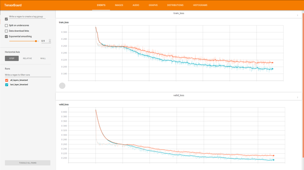
So I’ve run the model with all binary units and only with last binary unit. And it seems that model with only last layer binarized trains better. After a while, I note that this approach was already proposed in the paper, but I somehow miss this.
So let’s stop with the last layer binarized and try different train approaches. To build model that will train only pair of layers we need train two layers model, save it, build new model with one more layer, load pre-trained first two layers weights/biases and continue train last two layers (code). During implementation I’ve met some trouble - tensorflow have no method to initialize all not initialized previously variables method. Maybe I just didn’t find this. So I’ve finished with approach when I directly send variable that should be restored and variables that should be initialized.
# restore previous variables
restore_vars_dict = self._get_restored_variables_names()
restorer = tf.train.Saver(restore_vars_dict)
restorer.restore(sess, self.saves_path)

# initialize not restored variables
new_variables = self._get_new_variables_names()
sess.run(tf.initialize_variables(new_variables))
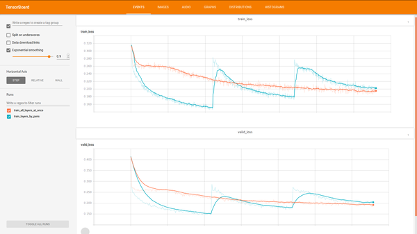
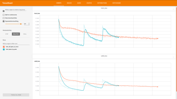
After testing seems that both training approaches converge to approximately same error. But some another cool stuff - the model that was trained by pair lairs trains faster in time.
So we stop with RBM trained with only last layer binarized and with two layers only strategy.
Build autoencoder from RBM
After getting pre-trained weights from RMB, it’s time to build autoencoder for fine tuning. To get encoding layer output as much as possible binarized as per paper advice we add Gaussian noise before layer. To simulate deterministic noise behavior, noise generated for each input prior training and not changed during training. Also, we want compare autoencoder loaded from RBM weights with self-initialized usual autoencoder. Code for autoencoder
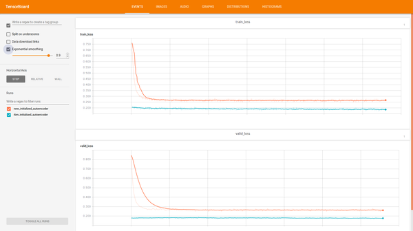
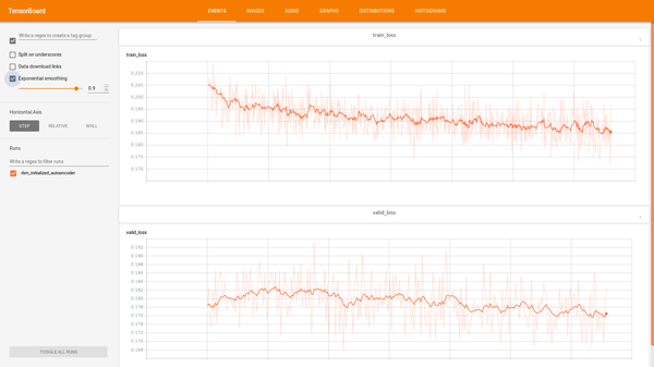
It seems that RBM initialized autoencoder continue training, but newly initialized autoencoder with same architecture after a while stuck at some point.
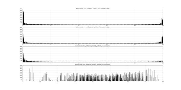
Also, I’ve trained two autoencoders without Gaussian noise. Now we can see through distribution what embedding most similar to binary (code for visualization):
We can see that RBM based autoencoder with Gaussian noise works better than other for our purposes.
Validation
To validate received embeddings I generate them for test and train sets for such networks:
- Initial MNIST(without embedding at all)
- RBM with the last layer binarized and trained by pairs
- Autoencoder based on RBM with Gaussian noise
- Newly initialized autoencoder with Gaussian noise
and use two validation approaches:
Train SVM with the train set and measure accuracy on the test set. SVM was used from sklearn with ‘rbf’ kernel with no max_iter == 50. Results table were generated with this code
| notes | accuracy | prec | f_score | recall |
|---|---|---|---|---|
| default mnist dataset | 0.446 | 0.647 | 0.460 | 0.454 |
| rbm: train_layers_by_pairs last_layer_binarized | 0.455 | 0.450 | 0.446 | 0.453 |
| autoencoder: rbm_initialized_model with_Gaussian_noise | 0.499 | 0.500 | 0.493 | 0.494 |
| autoencoder: new_initialized_model with_Gaussian_noise | 0.100 | 0.098 | 0.095 | 0.099 |
With Hamming distance or dot product find ten most similar pictures/embeddings to provided one and check how many labels are the same to the submitted array label. Code to check distance accuracies.
| notes | hamming accuracy | hamming time_cons | dot_product accuracy | dot_product time_cons |
|---|---|---|---|---|
| default mnist dataset | 0.910 | 180.4 | 0.916 | 528.8 |
| rbm: train_layers_by_pairs last_layer_binarized | 0.633 | 28.6 | 0.638 | 60.2 |
| autoencoder: rbm_initialized_model with_Gaussian_noise | 0.583 | 28.9 | 0.563 | 61.6 |
| autoencoder: new_initialized_model with_Gaussian_noise | 0.099 | 29.8 | 0.099 | 64.6 |
Conclusion
As we can see embeddings can save some strong features, that can be used for future clusterization very well. But these features are not linearly correlated - so when we measure accuracy for most similar embeddings, we get results worse than when we use full MNIST images. Of course, maybe autoencoder should be trained with another learning rate/longer, but this is the task for future research.
At the same time, we confirmed that training autoencoders from pre-trained RBMs weights are right to approach - the network will pass local optimization minimum and not stack at some point during training.
Training params
For RBM training such params were used network was trained with:
- epochs = 6
- learning rate = 0.01
- batch size = 100
- shuffle batches = True
- gibbs sampling steps = 1
- layers quantity = 3
- layers shapes(including input layer) = [784, 484, 196, 100]
For autoencoder learning rate was changed to 1.0 because of another optimization rule.
Comments
Comments powered by Disqus