General ML Notes
This notes based on Neural Networks and Deep Learning and Coursera ML Courses. They may seems to be some way unstructured, but work still in progress, so please be patient.
Contents:
Ֆ General Approach
- Define network architecture
- Choose right cost function
- Calculate gradient descent if necessary
- Train, tune hyperparameters.
Ֆ Part I
An idea of stochastic gradient descent is to estimate the gradient \(\nabla C\) by computing \(\nabla Cx\) for a small sample of randomly chosen training inputs, not for all inputs as usual gradient descent do. For this stochastic gradient descent take small number of m randomly chosen training inputs. We’ll label those random training inputs \(X1,X2,\ldots ,Xm\) and refer to them as a mini-batch. So now gradinet can be computed as:
Ֆ Part II
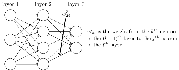
image from this book
Elementwise product of the two vectors denoted as \(s \odot t\) and can be called sometimes Hadamard product or Schur product. Her is an example:
In tensorflow you should distinguish usual matrix multiplication and hadamard product
# W, Q - some matrices

# matrix multiplication
res = math_ops.matmul(W, Q)

# hadamard product
res = W * Q
Ֆ Part III
Regularization
Weight decay or L2 regularization
The idea of L2 regularization is to add an extra term to the cost function, a term called the regularization term.
Where \(C_0\) is the original cost, second part - regularization term itself (namely the sum of the squares of all the weights in the network). This is scaled by a factor \(\frac{\lambda}{2n}\), where \(\lambda > 0\) is known as regularization parameter, and \(n\) is, as ususal, the size of our training set.
Weight decay factor - \(1-\frac{\eta\lambda}{n}\). So during training on larger dataset we should change \(\lambda\) with respect to learning rate and size of training set.
How to choose a neural network’s hyper-parameters?
Broad strategy
- Simplify the model
- Reduce classification classes
- Reduce training/validation data
- Increase frequency of monitoring
- With such updates you may try to find required hyper-parameters very fast
Learning rate (η)
- Estimate the threshold value for η at which the cost on the training data immediately begins decreasing, instead of oscillating or increasing.
- After you likely want to use value of η that is smaller, say, a factor of two bellow the threshold.
Using early stopping
A better rule is to terminate if the best classification accuracy doesn’t improve for quite some time. For example we might elect to terminate if the classification accuracy hasn’t improved during the last ten epochs.
Learning rate schedule
We need choose when learning rate should be decreased and by what rule. Some of existing rules are:
- Step decay - reduce learning rate by some factor.
- Exponental decay - \(\alpha = \alpha_0 e^{-k t}\), where \(\alpha_0, k\) are hyperparameters and \(t\) is the iteration number (but you can also use units of epochs).
- 1/t decay - \(\alpha = \alpha_0 / (1 + k t )\), where \(\alpha_0, k\) are hyperparameters and \(t\) is the iteration number.
Also you may checked predefined learning schedules at tensorflow. But prior to use learning rate schedule it’s better to get best performed model with fixed learning rate.
Mini-batch size
Wights updates for online learning can be declarated as:
For case of mini-batch of size 100 we get:
With this we may increase learning rate by a factor 100 and updated rules become:
With choosing mini-batch size we shouldn’t update any others hyper-parameters, only learning rate should be checked. After we may try different mini-batches sizes, scaling learning rate as required and choose what validation accuracy updates faster at real time(not related to epochs) in order to maximize our model overall speed.
Automated techniques
For automated hyper-parameters choose we can use grid search or something like Bayesian approach (source code)
Futher reading
- Practical recommendations for gradient-based training of deep architectures
- Efficient BackProp
- Neural Networks: Tricks of the Trade (you may try not to use hwole book, but search for some articles from its authors)
Ֆ Evaluation of algorithm
What we should do:
- Split the dataset into three portions: train set, validate set and test set, in a proportion 3:1:1.
- When the number of examples m increase, the cost \({J_{test}}\) increases, while \({J_{val}}\) decrease. When m is very large, if \({J_{test}}\) is about equal to \({J_{val}}\) the algorithm may suffer from large bias(underfiting), while if there is a gap between \({J_{test}}\) and \({J_{val}}\) the algorithm may suffer from large variance(overfitting).
- To solve the problem of large bias, you may decrease \({\rm{\lambda }}\) in regularization, while increase it for the problem of large variance.
- To evaluate the performance of a classification algorithm, we can use the value: precision, recall and F1.
Precision:
Recall:
F1:
Ֆ Overfiting and underfitting
High bias is underfitting and high variance is overfitting.
For understanding what exactly mean Bias and Variance you may check this or this cool articles.
Next notes based on awesome Andre Ng lecture
During training as usual you split your data on train, validation and test sets. Note: You should keep your validation/test data the same for model you want to compare. After measuring errors you can get some results. In this case difference between human error (how human perform such task) and train error will be bias. On the other hand, difference between train error and validation error will be variance.
In such case you should consider this methods
Solutions inside blue boxes should be applied as first approach.
But sometimes you may have a lot of data from one domain, but test data comes from another. In this case validation and test data should be from the same domain. Also you may consider get validation data also from large domain. But it should be additional validation(say train-valid). Let’s see an example.
In this case we receive another correlation between errors:
And solution algorithm will be a little bit more longer: